The Definitive Guide for Vlookup Example

Usage VLOOKUP when you need to locate things in a table or a range by row. For instance, seek out a cost of an auto component by the part number, or discover an employee name based on their staff member ID. In its simplest form, the VLOOKUP function claims: =VLOOKUP(What you intend to search for, where you wish to try to find it, the column number in the variety consisting of the worth to return, return an Approximate or Specific match-- indicated as 1/TRUE, or 0/FALSE).

Use the VLOOKUP feature to search for a worth in a table. Syntax VLOOKUP (lookup_value, table_array, col_index_num, [range_lookup] For example: =VLOOKUP(A 2, A 10: C 20,2, TRUE) =VLOOKUP("Fontana", B 2: E 7,2, FALSE) =VLOOKUP(A 2,'Customer Particulars'! A: F,3, FALSE) Argument name Summary lookup_value (needed) The worth you wish to seek out. The value you intend to search for have to be in the very first column of the series of cells you specify in the table_array disagreement.

Lookup_value can be a value or a reference to a cell. table_array (needed) The variety of cells in which the VLOOKUP will look for the lookup_value and also the return value. You can use a called array or a table, and also you can make use of names in the argument instead of cell references.

The cell array additionally needs to consist of the return worth you wish to find. Learn how to choose ranges in a worksheet. col_index_num (required) The column number (starting with 1 for the left-most column of table_array) which contains the return worth. range_lookup (optional) A sensible worth that defines whether you want VLOOKUP to discover an approximate or a specific match: Approximate suit - 1/TRUE thinks the initial column in the table is arranged either numerically or alphabetically, and will after that search for the closest worth.

For instance, =VLOOKUP(90, A 1: B 100,2, TRUE). Precise suit - 0/FALSE look for the specific value in the first column. As an example, =VLOOKUP("Smith", A 1: B 100,2, FALSE). There are four pieces of information that you will certainly require in order to construct the VLOOKUP syntax: The worth you desire to search for, likewise called the lookup value.

The Facts About Vlookup Example Revealed

Keep in mind that the lookup worth need to constantly be in the initial column in the range for VLOOKUP to function correctly. For instance, if your lookup value is in cell C 2 after that your variety ought to start with C. The column number in the variety that has the return worth. As an example, if you define B 2:D 11 as the array, you should count B as the first column, C as the 2nd, and so on.

If you don't specify anything, the default worth will always be REAL or approximate match. Currently place all of the above with each other as follows: =VLOOKUP(lookup worth, array containing the lookup value, the column number in the range containing the return value, Approximate match (TRUE) or Exact suit (FALSE)). Here are a couple of instances of VLOOKUP: Issue What failed Incorrect worth returned If range_lookup holds true or omitted, the very first column needs to be sorted alphabetically or numerically.

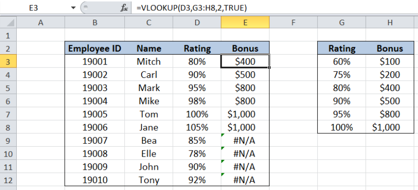
Either type the very first column, or utilize FALSE for a specific suit. #N/ A in cell If range_lookup is REAL, after that if the value in the lookup_value is smaller than the smallest value in the initial column of the table_array, you'll get the #N/ A mistake worth. If range_lookup is FALSE, the #N/ An error value indicates that the precise number isn't found.

#REF! in cell If col_index_num is more than the number of columns in table-array, you'll obtain the #REF! error worth. For even more details on fixing #REF! mistakes in VLOOKUP, see Just how to fix a #REF! error. #VALUE! in cell If the table_array is much less than 1, you'll obtain the #VALUE! error worth.

#NAME? in cell The #NAME? error worth typically means that the formula is missing quotes. To seek out a person's name, make certain you make use of quotes around the name in the formula. As an example, get in the name as "Fontana" in =VLOOKUP("Fontana", B 2: E 7,2, FALSE). For additional information, see How to correct a #NAME! mistake.

Vlookup Can Be Fun For Anyone

Find out just how to make use of outright cell referrals. Don't store number or day worths as text. When searching number or day worths, be sure the data in the first column of table_array isn't kept as message values. Otherwise, VLOOKUP may return an inaccurate or unforeseen value. Arrange the first column Kind the very first column of the table_array prior to utilizing VLOOKUP when range_lookup is TRUE.

An inquiry mark matches any type of solitary character. An asterisk matches any sequence of characters. If you desire to discover a real inquiry mark or asterisk, kind a tilde (~) in front of the character. For example, =VLOOKUP("Fontan?", B 2: E 7,2, FALSE) will certainly look for all circumstances of Fontana with a last letter that might differ.

When searching message worths in the initial column, see to it the information in the initial column doesn't have leading rooms, tracking areas, irregular use straight (' or") and curly (' or ") quote marks, or nonprinting personalities. In these instances, VLOOKUP could return an unanticipated value.

You can constantly ask a specialist in the Excel User Voice. Quick Recommendation Card: VLOOKUP refresher course Quick Reference Card: VLOOKUP repairing tips You Tube: VLOOKUP video clips from Excel neighborhood specialists Whatever you need to find out about VLOOKUP Just how to deal with a #VALUE! mistake in the VLOOKUP function How to deal with a #N/ A mistake in the VLOOKUP feature Overview of solutions in Excel Exactly how to prevent damaged formulas Detect errors in solutions Excel features (indexed) Excel functions (by group) VLOOKUP (cost-free sneak peek).

To compute shipping price based on weight, you can utilize the VLOOKUP function. In the instance revealed, the formula in F 8 is: =VLOOKUP(F 7, B 6: C 10,2,1)* F 7 This formula uses the weight to locate the proper "cost per kg" then ... To bypass result from VLOOKUP, you can nest VLOOKUP in the IF function.

vlookup in excel youtube malayalam excel vlookup not working vlookup in excel col_index_num